 digest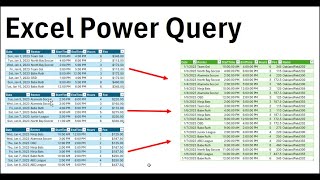
Short Summary
Main recommendation: Use Power Query's Excel.CurrentWorkbook function to consolidate multiple same-structure Excel tables into one master table, rather than using older array formulas. The video also shows how to avoid the recursion (double-records) problem caused by refreshing the exported table, and how to skip the master table and load the data straight into a PivotTable.
Key Points
- Power Query (available since Excel 2013) with Excel.CurrentWorkbook imports all tables in the workbook, stacking them on top of one another, replacing the older array-formula approach.
- Excel.CurrentWorkbook also imports other objects such as defined names and lookup tables, so those must be filtered out explicitly.
- Exporting the query result to the worksheet creates an Excel table that Power Query then re-reads on refresh, causing records to double (the "ghost row" / recursion problem).
- The fix is to filter out the master table's own name in a Filter Rows step, so future refreshes do not re-import it.
- Future tables added to the workbook are picked up automatically, as long as they share the same column count and field names.
Details Worth Noting
- Concrete instructions:
- Press Alt+F12 to open the Power Query Editor.
- Find the right-click key on your keyboard and press it, then press G (the keyboard shortcut for From Table/Range, which uses Excel.CurrentWorkbook).
- In the formula bar, delete the lookup portion so the code reads just Excel.CurrentWorkbook.
- In the drop-down, uncheck the defined name and any non-table objects (such as the lookup table) so they are excluded.
- Use the Expand button to expand the Content column and keep all columns, not the original "Content" column name.
- Select the first date/time columns, shift-click the last one, and use Transform > Detect Data Types, then manually change data types (for example, Date for Start Time and Time for End Time).
- Name the query "Master Fee Table".
- To prevent doubling, go to the Filter Rows step, copy the Name filter condition, and combine it with the existing filter using the lowercase "and" operator, then press Enter.
- To build a PivotTable: select a cell, Insert PivotTable (Alt, N, V, T), use Existing worksheet, and click OK.
- To analyze tables without a master table: clear all (Alt, E, A, A), keep the query as "connection only," then right-click and choose Load To, selecting PivotTable.
- Each source table must have the same number of columns and identical field names, or the consolidation will break.
- New rows typed directly under the Excel table auto-extend formatting (for example, using Control+apostrophe to copy the cell above); PivotTables then refresh with a right-click.
- The video notes a pitfall: a stray number-format change (250 showing with the wrong format) carried down from typing in a new row; the speaker said he wasn't sure exactly how it happened and left it as an example of the issue, without confirming a fix was shown.
Bottom Line
Excel.CurrentWorkbook in Power Query is the simplest way to stack same-structure tables, but you must filter out the master table's own name to avoid doubled records, and loading the query as connection-only directly to a PivotTable is an option when a master table is unnecessary.


