 digest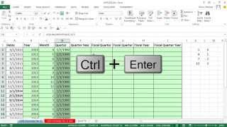
Short Summary
Main recommendation: To convert dates into quarters, use CEILING on the month number with a significance of 3 and divide by 3; for fiscal quarters and years that don't match the calendar, use a LOOKUP table or a month-based IF formula and subtract one from the year for the fiscal months 1–3. The video demonstrates these approaches in Excel, with the IF-based formula noted as also working in Power Pivot.
Key Points
- CEILING(month, 3) / 3 returns calendar quarters: months 1–3 = Q1, 4–6 = Q2, 7–9 = Q3, 10–12 = Q4.
- For a quarter and year label, the video joins "Q", the quarter, " - ", and the year with ampersands (e.g., "Q2 2013").
- For fiscal quarters, a LOOKUP table maps months to fiscal quarters; the presenter credits Barry Houdini for the technique.
- Power Pivot lacks some Excel functions, so an IF-based formula is offered as an alternative to CEILING.
- A fiscal year starting in a prior-calendar-year month needs the year reduced by one for the fiscal months 1, 2, and 3.
Details Worth Noting
Concrete instructions:
- Calendar quarter: enter =CEILING(MONTH(date),3)/3 and fill down; check that the result is formatted as General (Control Shift ~ removes date formatting).
- Quarter and year label: combine "Q" & quarter & " - " & year in one formula.
- Fiscal quarter via LOOKUP: build a two-column table (month numbers in column 1, fiscal quarters in column 2) and use =LOOKUP(month, table_column, result_column) with the table range locked by F4. LOOKUP performs an approximate match and takes results from the last column of the table.
- Hardcoded fiscal table: highlight the array and press F9 to see its array constant form (curly brackets, commas for columns, semicolons for rows), then enter it directly as an array constant to avoid a separate table.
- Power Pivot–friendly quarter: =IF(month<4, 4, CEILING(month,3)/3 - 1), filled down.
- Fiscal year adjustment: =year - (month<4), which subtracts one only for months 1–3 because TRUE converts to 1 in math operations; Alt, M, V evaluates the formula step by step.
- Combine the fiscal quarter and the adjusted fiscal year with the same "Q" concatenation pattern.
- Example result: a month-1, 2014 date returns "Q4 2013" once the fiscal quarter and adjusted fiscal year are combined.
Bottom Line
Calendar quarters are straightforward with CEILING, but fiscal periods that cross the calendar year require either a lookup table or an IF-based formula combined with subtracting one from the year for the early fiscal months.


