digest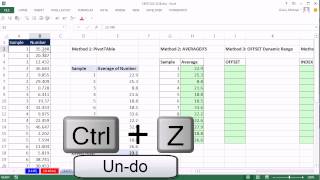
Short Summary
Main recommendation: For averaging each sample, use a PivotTable (fast, but needs manual refresh) or AVERAGEIFS (updates automatically) when there is a sample column, and use AVERAGE wrapped around an OFFSET-built dynamic range when there is no sample column and data repeats every three items.
Key Points
- A PivotTable gives the fastest result: it lists each unique sample and its average, but it must be refreshed after the source data changes.
- AVERAGEIFS averages the numbers whose sample value matches the criteria cell, and its formulas update automatically when data changes.
- Pivot table averages and formulas can show different decimals; number formatting only changes the display, so ROUND can be used if the underlying values need to be rounded.
- When samples are not labeled in a column, OFFSET can pick out each group of three values by moving down the list in steps of three.
- OFFSET is a volatile function, so it may slow large workbooks, and INDEX is suggested as an alternative for dynamic ranges.
Details Worth Noting
- Concrete instructions:
- PivotTable: Click a single cell in the data, insert a PivotTable (keyboard shortcut Alt, N, V in 2013; Alt, N, V, T in 2010 and 2007), and place it on the existing sheet in an empty area so it does not overwrite other data. Drag the sample number field to Rows and the number field to Values. Right-click the value, choose Value Field Settings, select Average, open Number Formatting, choose Number with one decimal place, and click OK. To make the header clearer, go to Design, Report Layout, Show in Tabular Form. After changing source data, right-click the PivotTable and choose Refresh.
- AVERAGEIFS: Enter =AVERAGEIFS(average range, criteria range, criteria). Select the top value cell, press Control+Shift+Down Arrow to extend to the bottom, and press F4 to lock the range. Use the same method for the criteria range, then use the sample number cell as the criteria. Press Control+Enter and double-click to fill down.
- Rounding AVERAGEIFS results: Press F2 to edit the formula, wrap it in ROUND, and type 1 as the digit count to round to one decimal place. Press Control+Enter to fill down.
- OFFSET without a sample column: Use =ROW(J$5)-1 style counting, multiply by 3, then add 1 to produce starting positions 1, 4, 7, and so on. Then build =OFFSET(first field name cell locked with F4, starting position, , 3) to return three rows at a time, and wrap that in AVERAGE. Use F9 on a selected OFFSET formula to check the values it returns.
- The speaker notes that the sample column and criteria are what let AVERAGEIFS and the PivotTable group values correctly.
- The speaker recommends INDEX instead of OFFSET for very large data sets or many formulas, but does not demonstrate it in this video.
- The video is part of the excelisfun Magic Trick series.
Bottom Line
Use a PivotTable or AVERAGEIFS when samples are labeled, and reserve OFFSET-based AVERAGE for data without a sample column, keeping the volatility trade-off in mind for large workbooks.