digest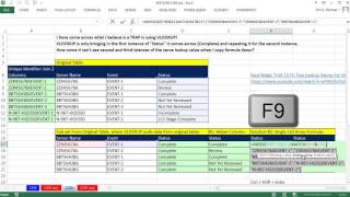
Short Summary
Main recommendation: To use VLOOKUP when a lookup value appears more than once, create a helper column that joins server name and event with the ampersand (&), then look up that combined value. When a helper column isn't possible, a single-cell INDEX-MATCH formula with array operations is the alternative, and wrapping the array inside INDEX avoids needing Control+Shift+Enter.
Key Points
- VLOOKUP with exact match (FALSE or 0) only returns the first match when duplicate values exist in the lookup column, so the video's example returned only Event 1 for servers with multiple events.
- A combined key (server name & event) is unique per row, which makes the lookup work correctly.
- Without a helper column, MATCH can find the row number of a combined server-and-event array, and INDEX can return the status value from that row.
- The video presents a single-cell array formula that requires Control+Shift+Enter, which shows curly brackets in the formula bar and returns an error if omitted.
- The video says the INDEX array argument can handle array operations without Control+Shift+Enter when the row number is left empty, which pulls all rows at once.
- He says the helper column with VLOOKUP is usually the fastest and easiest approach, and says the nested INDEX-MATCH (INDEX wrapping the array, no Control+Shift+Enter) is probably the one he would use for a single-cell formula.
Details Worth Noting
- Concrete instructions:
- Helper column method: in a new column, enter the server name joined to the event with & (for example, server name & event), fill it down, then in VLOOKUP use the same join as the lookup value (server name & event) with the helper table's first column, the table range extended to include the helper column, column index 4 for the status column, and FALSE or 0 for exact match.
- Single-cell method: in the formula, use INDEX with the status column as the array and MATCH as the row number. Set MATCH's lookup value to server name & event, and its lookup array to (server name column & event column), with the lookup array range locked using F4 (absolute references). Use MATCH's match_type as 0 for exact match.
- Array entry: when the array operation is entered directly in MATCH's lookup array, press Control+Shift+Enter to enter it as an array formula; otherwise Excel returns an error.
- No-keystroke variant: wrap the array operation inside a second INDEX, leave its row number argument empty, and press Control+Enter (no Control+Shift+Enter needed).
- Verify with F9 on the lookup value or the lookup array to confirm the joined values or the row number are calculating correctly.
- The video references a companion video, Excel Magic Trick 1174, which covers six different ways to solve this problem.
- The video's example data uses server names with multiple events, with a status column returned as the fourth column of the lookup table.
Bottom Line
For duplicate lookup keys, the video's clearest path is a helper column joining the fields with &, and the single-cell INDEX-MATCH approach works when a helper column isn't possible.