 digest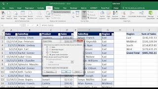
Short Summary
Main recommendation: Use Power Query's Merge feature (a Left Outer join) to combine two Excel tables into one connected query, then build a PivotTable from that merged query to summarize sales by region. He mentions VLOOKUP or a Data Model relationship as alternatives, but shows the Merge approach as the method for this video.
Key Points
- Both source ranges must first be converted to official Excel tables (Ctrl+T), which Power Query requires.
- The two tables are linked on the shared "Sales Rep" column, and the lookup table's Region column is pulled into the sales table.
- The merged query is loaded as "Only Create a Connection," so the combined data is not duplicated on the sheet.
- The resulting PivotTable uses the merged query as an external data source, with Region in Rows and Sales in Values.
Details Worth Noting
- Concrete instructions:
- Select a single cell in each range and press Ctrl+T to convert it to an Excel table. Name each table in Table Design > Table Name (the video names the lookup table D_Sales_Rep and the sales table F_Sales).
- Select a cell in the sales table, go to Data > Get & Transform > From Table/Range, and let it open in the Query Editor.
- Fix data types by clicking the type icon and choosing Currency for amounts and Date for dates, then choose "Replace Current."
- Repeat From Table/Range for the second table, then click Close & Load > Close & Load To, and select "Only Create a Connection" for each query.
- Go to Get Data > Combine Queries > Merge. Select F_Sales and the Sales Rep column, select D_Sales_Rep and its Sales Rep column, and choose Left Outer join so all sales records are kept.
- Rename the new merged column to "Region," then click the expand button. Uncheck "Use original column name as prefix," and uncheck Select All, keeping only Region to avoid duplicates. Fix the data type if needed.
- Click Close & Load To > Only Create a Connection, then rename the query (the video uses Sales_Table) via right-click > Properties.
- Insert a PivotTable with Alt, N, V, choose "Use an external data source," select Connection, and pick the Sales_Table query.
- Drag Region to Rows and Sales to Values, then set Design > Report Layout > Show in Tabular Form and apply Currency number formatting.
- The video notes that the Excel version and ribbon layout may differ; the presenter uses Excel 2016 and mentions a recent update changed the Get & Transform and Close & Load dialogs.
- The new Close & Load To dialog merges the older Import Data and Load To options; "Add to the Data Model" is not used in this method.
- Alternatives the presenter mentions but does not use here are a VLOOKUP helper column or Data Model relationships.
Bottom Line
Power Query's Merge is a clean way to produce a single combined table that feeds a PivotTable without duplicating data on the sheet.


